Understanding Multimodal LLMs
An introduction to the main techniques and latest models
It was a wild two months. There have once again been many developments in AI research, with two Nobel Prizes awarded to AI and several interesting research papers published.
Among others, Meta AI released their latest Llama 3.2 models, which include open-weight versions for the 1B and 3B large language models and two multimodal models.
In this article, I aim to explain how multimodal LLMs function. Additionally, I will review and summarize roughly a dozen other recent multimodal papers and models published in recent weeks (including Llama 3.2) to compare their approaches.
(To see a table of contents menu, click on the stack of lines on the left-hand side.)

But before we begin, I also have some exciting news to share on the personal front! My book, "Build A Large Language Model (From Scratch)", is now finally available on Amazon!

Writing this book was a tremendous effort, and I’m incredibly grateful for all the support and motivating feedback over the past two years—especially in these last couple of months, as so many kind readers have shared their feedback. Thank you all, and as an author, there is nothing more motivating than to hear that the book makes a difference in your careers!
For those who have finished the book and are eager for more, stay tuned! I’ll be adding some bonus content to the GitHub repository in the coming months.
P.S. If you have read the book, I'd really appreciate it if you could leave a brief review; it truly helps us authors!
1. Use cases of multimodal LLMs
What are multimodal LLMs? As hinted at in the introduction, multimodal LLMs are large language models capable of processing multiple types of inputs, where each "modality" refers to a specific type of data—such as text (like in traditional LLMs), sound, images, videos, and more. For simplicity, we will primarily focus on the image modality alongside text inputs.
A classic and intuitive application of multimodal LLMs is image captioning: you provide an input image, and the model generates a description of the image, as shown in the figure below.

Of course, there are many other use cases. For example, one of my favorites is extracting information from a PDF table and converting it into LaTeX or Markdown.
2. Common approaches to building multimodal LLMs
There are two main approaches to building multimodal LLMs:
Method A: Unified Embedding Decoder Architecture approach;
Method B: Cross-modality Attention Architecture approach.
(By the way, I don’t believe official terms for these techniques exist yet, but let me know if you’ve come across any. For instance, briefer descriptions may be "decoder-only" and "cross-attention-based" approaches.)
As shown in the figure above, the Unified Embedding-Decoder Architecture utilizes a single decoder model, much like an unmodified LLM architecture such as GPT-2 or Llama 3.2. In this approach, images are converted into tokens with the same embedding size as the original text tokens, allowing the LLM to process both text and image input tokens together after concatenation.
The Cross-Modality Attention Architecture employs a cross-attention mechanism to integrate image and text embeddings directly within the attention layer.
In the following sections, we will explore how these methods work on a conceptual level. Then, we will look at recent research papers on multimodal LLMs to see how they are applied in practice.
2.1 Method A: Unified Embedding Decoder Architecture
Let’s begin with the unified embedding decoder architecture, illustrated again in the figure below.

In the unified embedding-decoder architecture, an image is converted into embedding vectors, similar to how input text is converted into embeddings in a standard text-only LLM.
For a typical text-only LLM that processes text, the text input is usually tokenized (e.g., using Byte-Pair Encoding) and then passed through an embedding layer, as shown in the figure below.

2.1.1 Understanding Image encoders
Analogous to the tokenization and embedding of text, image embeddings are generated using an image encoder module (instead of a tokenizer), as shown in the figure below.
What happens inside the image encoder shown above? To process an image, we first divide it into smaller patches, much like breaking words into subwords during tokenization. These patches are then encoded by a pretrained vision transformer (ViT), as shown in the figure below.
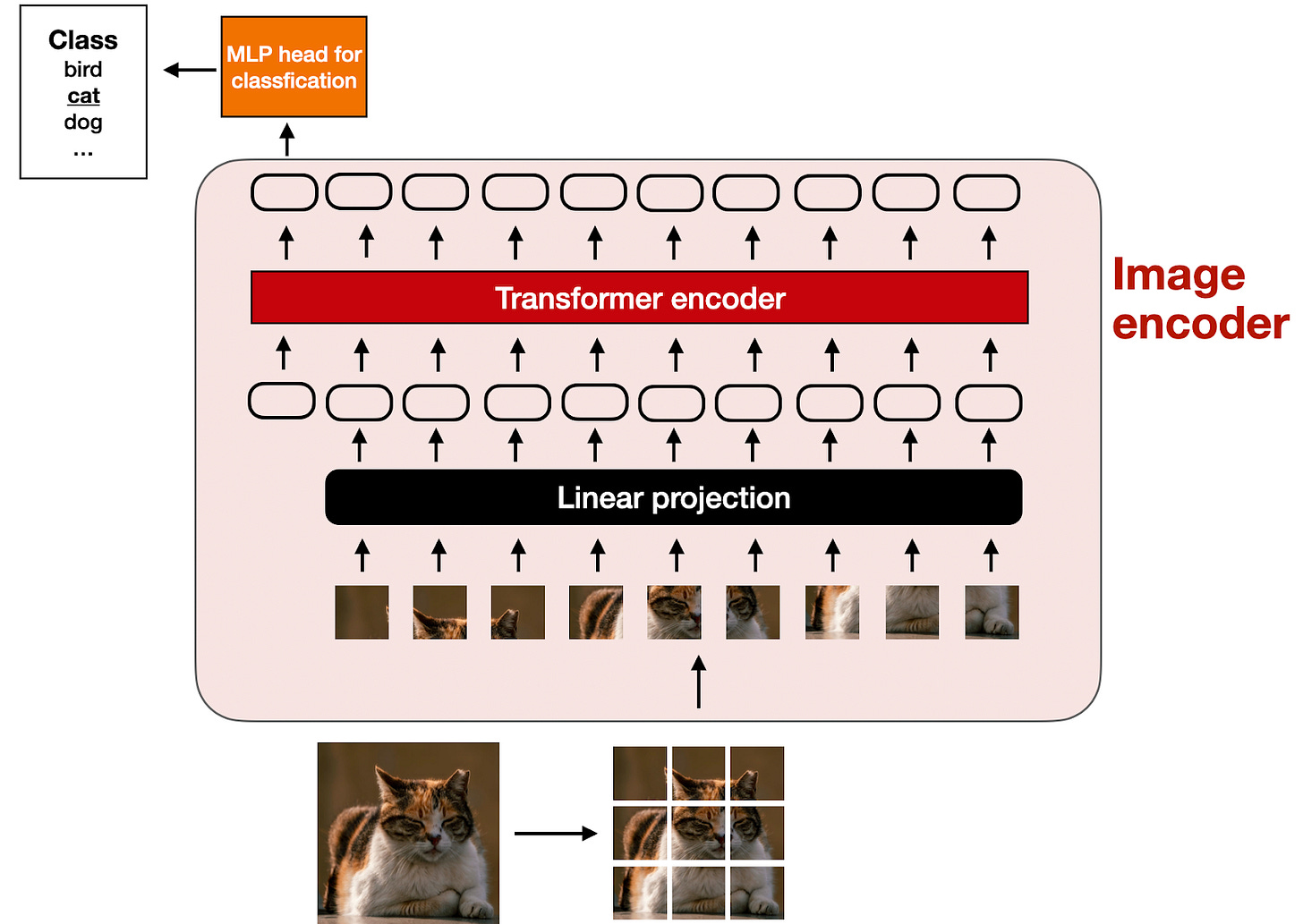
Note that ViTs are often used for classification tasks, so I included the classification head in the figure above. However, in this case, we only need the image encoder part.
2.1.2 The role of the linear projection module
The "linear projection" shown in the previous figure consists of a single linear layer (i.e., a fully connected layer). The purpose of this layer is to project the image patches, which are flattened into a vector, into an embedding size compatible with the transformer encoder. This linear projection is illustrated in the figure below. An image patch, flattened into a 256-dimensional vector, is up-projected to a 768-dimensional vector.

For those who prefer seeing a code example, In PyTorch code, we could implement the linear projection for the image patches as follows:
import torch


class PatchProjectionLayer(torch.nn.Module):

    def __init__(self, patch_size, num_channels, embedding_dim):
        super().__init__()
        self.patch_size = patch_size
        self.num_channels = num_channels
        self.embedding_dim = embedding_dim
        self.projection = torch.nn.Linear(
            patch_size * patch_size * num_channels, embedding_dim
        )

    def forward(self, x):

        batch_size, num_patches, channels, height, width = x.size()
        x = x.view(batch_size, num_patches, -1)  # Flatten each patch
        x = self.projection(x)  # Project each flattened patch
        return x


# Example Usage:
batch_size = 1
num_patches = 9  # Total patches per image
patch_size = 16  # 16x16 pixels per patch
num_channels = 3  # RGB image
embedding_dim = 768  # Size of the embedding vector

projection_layer = PatchProjectionLayer(patch_size, num_channels, embedding_dim)

patches = torch.rand(
    batch_size, num_patches, num_channels, patch_size, patch_size
)

projected_embeddings = projection_layer(patches)
print(projected_embeddings.shape)

# This prints
# torch.Size([1, 9, 768])
If you have read my Machine Learning Q and AI book by chance, you may know there are ways to replace linear layers with convolution operations that can be implemented to be mathematically equivalent. Here, this can be especially handy as we can combine the creation of patches and projection into two lines of code:
layer = torch.nn.Conv2d(3, 768, kernel_size=(16, 16), stride=(16, 16))

image = torch.rand(batch_size, 3, 48, 48)
projected_patches = layer(image)

print(projected_patches.flatten(-2).transpose(-1, -2).shape)
# This prints
# torch.Size([1, 9, 768])
2.1.3 Image vs text tokenization
Now that we briefly discussed the purpose of the image encoder (and the linear projection that is part of the encoder), let's return to the text tokenization analogy from earlier and look at text and image tokenization and embedding side by side, as depicted in the figure below.
As you can see in the figure above, I included an additional projector module that follows the image encoder. This projector is usually just another linear projection layer that is similar to the one explained earlier. The purpose is to project the image encoder outputs into a dimension that matches the dimensions of the embedded text tokens, as illustrated in the figure below. (As we will see later, the projector is sometimes also called adapter, adaptor, or connector.)

Now that the image patch embeddings have the same embedding dimension as the text token embeddings, we can simply concatenate them as input to the LLM, as shown in the figure at the beginning of this section. Below is the same figure again for easier reference.

By the way, the image encoder we discussed in this section is usually a pretrained vision transformer. A popular choice is CLIP or OpenCLIP.
However, there are also versions of Method A that operate directly on patches, such as Fuyu, which is shown in the figure below.

As illustrated in the figure above, Fuyu passes the input patches directly into a linear projection (or embedding layer) to learn its own image patch embeddings rather than relying on an additional pretrained image encoder like other models and methods do. This greatly simplifies the architecture and training setup.
2.2 Method B: Cross-Modality Attention Architecture
Now that we have discussed the unified embedding decoder architecture approach to building multimodal LLMs and understand the basic concept behind image encoding, let's talk about an alternative way of implementing multimodal LLMs via cross-attention, as summarized in the figure below.
In the Cross-Modality Attention Architecture method depicted in the figure above, we still use the same image encoder setup we discussed previously. However, instead of encoding the patches as input to the LLM, we connect the input patches in the multi-head attention layer via a cross-attention mechanism.
The idea is related and goes back to the original transformer architecture from the 2017 Attention Is All You Need paper, highlighted in the figure below.

Note that the original "Attention Is All You Need" transformer depicted in the figure above was originally developed for language translation. So, it consists of a text encoder (left part of the figure) that takes the sentence to be translated and generates the translation via a text decoder (right part of the figure). In the context of multimodal LLM, the encoder is an image encoder instead of a text encoder, but the same idea applies.
How does cross-attention work? Let's have a look at a conceptual drawing of what happens inside the regular self-attention mechanism.

In the figure above, x is the input, and Wq is a weight matrix used to generate the queries (Q). Similarly, K stands for keys, and V stands for values. A represents the attention scores matrix, and Z are the inputs (x) transformed into the output context vectors. (If this seems confusing, you may find a comprehensive introduction in Chapter 3 of my Build a Large Language Model from Scratch book helpful; alternatively, you may also find my article, Understanding and Coding Self-Attention, Multi-Head Attention, Cross-Attention, and Causal-Attention in LLMs helpful here.)
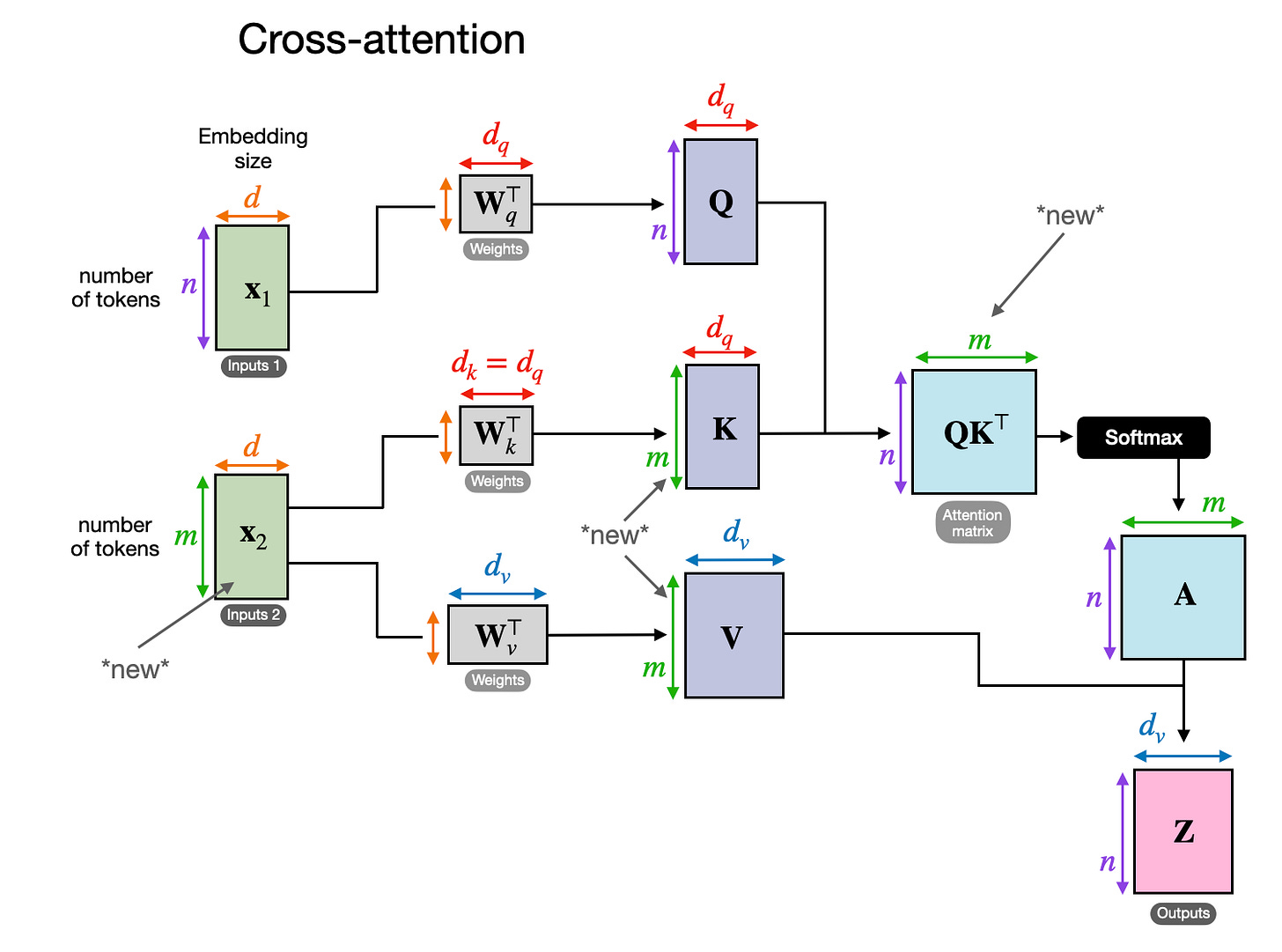
In cross-attention, in contrast to self-attention, we have two different input sources, as illustrated in the following figure.
As illustrated in the previous two figures, in self-attention, we work with the same input sequence. In cross-attention, we mix or combine two different input sequences.
In the case of the original transformer architecture in the Attention Is All You Need paper, the two inputs x1 and x2 correspond to the sequence returned by the encoder module on the left (x2) and the input sequence being processed by the decoder part on the right (x1). In the context of a multimodal LLM, x2 is the output of an image encoder. (Note that the queries usually come from the decoder, and the keys and values typically come from the encoder.)
Note that in cross-attention, the two input sequences x1 and x2 can have different numbers of elements. However, their embedding dimensions must match. If we set x1 = x2, this is equivalent to self-attention.
3. Unified decoder and cross-attention model training
Now that we have talked a bit about the two major multimodal design choices, let's briefly talk about how we deal with the three major components during model training, which are summarized in the figure below.

Similar to the development of traditional text-only LLMs, the training of multimodal LLMs also involves two phases: pretraining and instruction finetuning. However, unlike starting from scratch, multimodal LLM training typically begins with a pretrained, instruction-finetuned text-only LLM as the base model.
For the image encoder, CLIP is commonly used and often remains unchanged during the entire training process, though there are exceptions, as we will explore later. Keeping the LLM part frozen during the pretraining phase is also usual, focusing only on training the projector—a linear layer or a small multi-layer perceptron. Given the projector's limited learning capacity, usually comprising just one or two layers, the LLM is often unfrozen during multimodal instruction finetuning (stage 2) to allow for more comprehensive updates. However, note that in the cross-attention-based models (Method B), the cross-attention layers are unfrozen throughout the entire training process.
After introducing the two primary approaches (Method A: Unified Embedding Decoder Architecture and Method B: Cross-modality Attention Architecture), you might be wondering which is more effective. The answer depends on specific trade-offs.
The Unified Embedding Decoder Architecture (Method A) is typically easier to implement since it doesn't require any modifications to the LLM architecture itself.
The Cross-modality Attention Architecture (Method B) is often considered more computationally efficient because it doesn't overload the input context with additional image tokens, introducing them later in the cross-attention layers instead. Additionally, this approach maintains the text-only performance of the original LLM if the LLM parameters are kept frozen during training.
We will revisit the discussion on modeling performance and response quality in a later section, where we will discuss NVIDIA's NVLM paper.
This marks the end of what turned out to be a rather extensive introduction to multimodal LLMs. As I write this, I realize that the discussion has become lengthier than initially planned, which probably makes this a good place to conclude the article.
However, to provide a practical perspective, it would be nice to examine a few recent research papers that implement these approaches. So, we will explore these papers in the remaining sections of this article.
4. Recent multimodal models and methods
For the remainder of this article, I will review recent literature concerning multimodal LLMs, focusing specifically on works published in the last few weeks to maintain a reasonable scope.
Thus, this is not a historical overview or comprehensive review of multimodal LLMs but rather a brief look at the latest developments. I will also try to keep these summaries short and without too much fluff as there are 10 of them.
The conclusion section at the end of this has an overview that compares the methods used in these papers.
4.1 The Llama 3 Herd of Models
The Llama 3 Herd of Models paper (July 31, 2024) by Meta AI came out earlier this summer, which feels like ages ago in LLM terms. However, given that they only described but did not release their multimodal models until much later, I think it's fair to include Llama 3 in this list. (Llama 3.2 models were officially announced and made available on September 25.)
The multimodal Llama 3.2 models, which come in an 11-billion and 90-billion parameter version, are image-text models that use the previously described cross-attention-based approach, which is illustrated in the figure below.
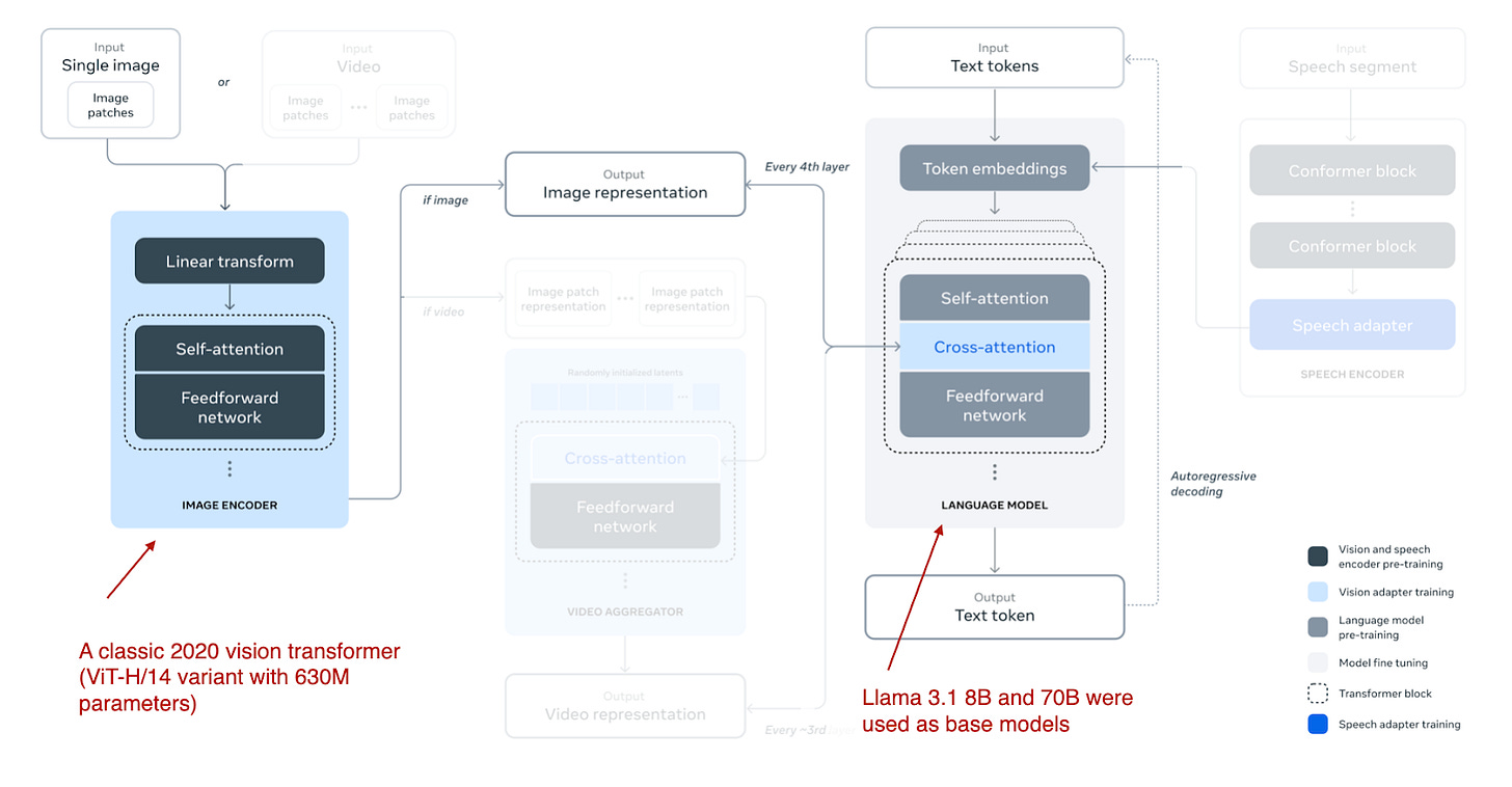
Note that while the figure also depicts video and speech as possible modalities, the models that were released as of this writing focus only on image and text.
Llama 3.2 uses the cross-attention-based approach. However, it differs a bit from what I wrote about earlier, namely that in multimodal LLM development, we usually freeze the image encoder and only update the LLM parameters during pretraining.
Here, the researchers almost take the opposite approach: they update the image encoder but do not update the language model's parameters. They write that this is intentional and done to preserve the text-only capabilities so that the 11B and 90B multimodal models can be used as drop-in replacements for the Llama 3.1 8B and 70B text-only model on text tasks.
The training itself is done in multiple iterations, starting with the Llama 3.1 text models. After adding the image encoder and projection (here called "adapter") layers, they pretrain the model on image-text data. Then, similar to the Llama 3 model text-only training (I wrote about it in an earlier article), they follow up with instruction and preference finetuning.
Instead of adopting a pretrained model such as CLIP as an image encoder, the researchers used a vision transformer that they pretrained from scratch. Specifically, they adopted the ViT-H/14 variant (630 million parameters) of the classic vision transformer architecture (Dosovitskiy et al., 2020). They then pretrained the ViT on a dataset of 2.5 billion image-text pairs over five epochs; this was done before connecting the image encoder to the LLM. (The image encoder takes 224×224 resolution images and divides them into a 14×14 grid of patches, with each patch sized at 16×16 pixels.)
As the cross-attention layers add a substantial amount of parameters, they are only added in every fourth transformer block. (For the 8B model, this adds 3B parameters, and for the 70B model, this adds 20 billion parameters.)
4.2 Molmo and PixMo: Open Weights and Open Data for State-of-the-Art Multimodal Models
The Molmo and PixMo: Open Weights and Open Data for State-of-the-Art Multimodal Models paper (September 25, 2024) is notable because it promises to open source not only the model weights but also the dataset and source code similar to the language-only OLMo LLM. (This is great for LLM research as it allows us to take a look at the exact training procedure and code and also lets us run ablation studies and reproduce results on the same dataset.)
If you are wondering why there are two names in the paper title, Molmo refers to the model (Multimodal Open Language Model), and PixMo (Pixels for Molmo) is the dataset.

As illustrated in the figure above, the image encoder employs an off-the-shelf vision transformer, specifically CLIP. The term "connector" here refers to a "projector" that aligns image features with the language model.
Molmo streamlines the training process by avoiding multiple pretraining stages, choosing instead a simple pipeline that updates all parameters in a unified approach—including those of the base LLM, the connector, and the image encoder.
The Molmo team offers several options for the base LLM:
OLMo-7B-1024 (a fully open model backbone),
OLMoE-1B-7B (a mixture-of-experts architecture; the most efficient model),
Qwen2 7B (an open-weight model that performs better than OLMo-7B-1024),
Qwen2 72B (an open-weight model and the best-performing model)
4.3 NVLM: Open Frontier-Class Multimodal LLMs
NVIDIA's NVLM: Open Frontier-Class Multimodal LLMs paper (September 17, 2024) is particularly interesting because, rather than focusing on a single approach, it explores both methods:
Method A, the Unified Embedding Decoder Architecture ("decoder-only architecture," NVLM-D), and
Method B, the Cross-Modality Attention Architecture ("cross-attention-based architecture," NVLM-X).
Additionally, they develop a hybrid approach (NVLM-H) and provide an apples-to-apples comparison of all three methods.

As summarized in the figure below, NVLM-D corresponds to Method A, and NVLM-X corresponds to Method B, as discussed earlier. The concept behind the hybrid model (NVLM-H) is to combine the strengths of both methods: an image thumbnail is provided as input, followed by a dynamic number of patches passed through cross-attention to capture finer high-resolution details.
In short, the research team find that:
NVLM-X demonstrates superior computational efficiency for high-resolution images.
NVLM-D achieves higher accuracy in OCR-related tasks.
NVLM-H combines the advantages of both methods.
Similar to Molmo and other approaches, they begin with a text-only LLM rather than pretraining a multimodal model from scratch (as this generally performs better). Additionally, they use an instruction-tuned LLM instead of a base LLM. Specifically, the backbone LLM is Qwen2-72B-Instruct (to my knowledge, Molmo used the Qwen2-72B base model).
While training all LLM parameters in the NVLM-D approach, they found that for NVLM-X, it works well to freeze the original LLM parameters and train only the cross-attention layers during both pretraining and instruction finetuning.
For the image encoder, instead of using a typical CLIP model, they use InternViT-6B, which remains frozen throughout all stages.
The projector is a multilayer perceptron rather than a single linear layer.
4.4 Qwen2-VL: Enhancing Vision-Language Model’s Perception of the World at Any Resolution
The previous two papers and models, Molmo and NVLM, were based on Qwen2-72B LLM. In this paper, the Qwen research team itself announces a multimodal LLM, Qwen2-VL: Enhancing Vision-Language Model's Perception of the World at Any Resolution (October 3rd, 2024).
At the core of this work is their so-called "Naive Dynamic Resolution" mechanism (the term "naive" is intentional and not a typo for "native," though "native" could also be fitting). This mechanism allows the model to handle images of varying resolutions without simple downsampling, enabling the input of images in their original resolution.

The native resolution input is implemented via a modified ViT by removing the original absolute position embeddings and introducing 2D-RoPE.
They used a classic vision encoder with 675M parameters and LLM backbones of varying sizes, as shown in the table below.
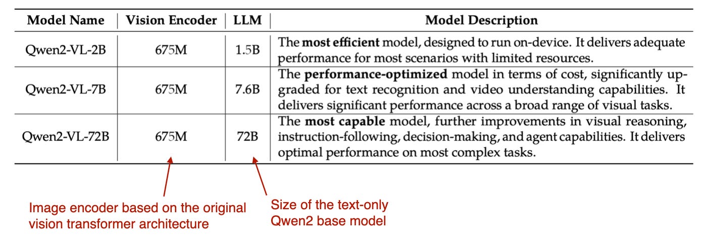
The training itself consists of 3 stages: (1) pretraining only the image encoder, (2) unfreezing all parameters (including LLM), and (3) freezing the image encoder and instruction-finetuning only the LLM.
4.5 Pixtral 12B
Pixtral 12B (September 17, 2024), which uses the Method A: Unified Embedding Decoder Architecture approach, is the first multimodal model from Mistral AI. Unfortunately, there is no technical paper or report available, but the Mistral team shared a few interesting tidbits in their blog post.
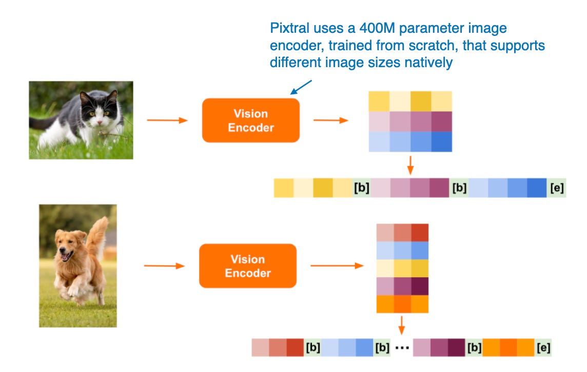
Interestingly, they chose not to use a pretrained image encoder, instead training one with 400 million parameters from scratch. For the LLM backbone, they used the 12-billion-parameter Mistral NeMo model.
Similar to Qwen2-VL, Pixtral also supports variable image sizes natively, as illustrated in the figure below.
4.6 MM1.5: Methods, Analysis & Insights from Multimodal LLM Fine-tuning
The MM1.5: Methods, Analysis & Insights from Multimodal LLM Fine-tuning paper (September 30, 2024) provides practical tips and introduces a mixture-of-experts multimodal model alongside a dense model similar to Molmo. The models span a wide size range, from 1 billion to 30 billion parameters.
The models described in this paper focuse on Method A, a Unified Embedding Transformer Architecture, which structures inputs effectively for multimodal learning.
In addition, the paper has a series of interesting ablation studies looking into data mixtures and the effects of using coordinate tokens.

4.7 Aria: An Open Multimodal Native Mixture-of-Experts Model
The Aria: An Open Multimodal Native Mixture-of-Experts Model paper (October 8, 2024) introduces another mixture-of-experts model approach, similar to one of the variants in the Molmo and MM1.5 lineups.
The Aria model has 24.9 billion parameters, with 3.5 billion parameters allocated per text token. The image encoder (SigLIP) has 438-million-parameters.
This model is based on a cross-attention approach with the following overall training procedure:
Training the LLM backbone entirely from scratch.
Pretraining both the LLM backbone and the vision encoder.
4.8 Baichuan-Omni
The Baichuan-Omni Technical Report (October 11, 2024) introduces Baichuan-Omni, a 7-billion-parameter multimodal LLM based on Method A: the Unified Embedding Decoder Architecture approach, as shown in the figure below.

The training process for Baichuan-Omni involves a three-stage approach:
Projector training: Initially, only the projector is trained, while both the vision encoder and the language model (LLM) remain frozen.
Vision encoder training: Next, the vision encoder is unfrozen and trained, with the LLM still frozen.
Full model training: Finally, the LLM is unfrozen, allowing the entire model to be trained end-to-end.
The model utilizes the SigLIP vision encoder and incorporates the AnyRes module to handle high-resolution images through down-sampling techniques.
While the report does not explicitly specify the LLM backbone, it is likely based on the Baichuan 7B LLM, given the model's parameter size and the naming convention.
4.9 Emu3: Next-Token Prediction is All You Need
The Emu3: Next-Token Prediction is All You Need paper (September 27, 2024) presents a compelling alternative to diffusion models for image generation, which is solely based on a transformer-based decoder architecture. Although it's not a multimodal LLM in the classic sense (i.e., models focused on image understanding rather than generation), Emu3 is super interesting as it demonstrates that it's possible to use transformer decoders for image generation, which is a task typically dominated by diffusion methods. (However, note that there have been other similar approaches before, such as Autoregressive Model Beats Diffusion: Llama for Scalable Image Generation.)

The researchers trained Emu3 from scratch and then used Direct Preference Optimization (DPO) to align the model with human preferences.
The architecture includes a vision tokenizer inspired by SBER-MoVQGAN. The core LLM architecture is based on Llama 2, yet it is trained entirely from scratch.
4.10 Janus: Decoupling Visual Encoding for Unified Multimodal Understanding and Generation
We previously focused on multimodal LLMs for image understanding and just saw one example for image generation with Emu 3 above. Now, the Janus: Decoupling Visual Encoding for Unified Multimodal Understanding and Generation paper (October 17, 2024) introduces a framework that unifies multimodal understanding and generation tasks within a single LLM backbone.
A key feature of Janus is the decoupling of visual encoding pathways to address the distinct requirements of understanding and generation tasks. The researchers argue that image understanding tasks require high-dimensional semantic representations, while generation tasks require detailed local information and global consistency in images. By separating these pathways, Janus effectively manages these differing needs.
The model employs the SigLIP vision encoder, similar to that used in Baichuan-Omni, for processing visual inputs. For image generation, it utilizes a Vector Quantized (VQ) tokenizer to handle the generation process. The base LLM in Janus is the DeepSeek-LLM with 1.3 billion parameters.

The training process for the model in this image follows three stages, as shown in the figure below.

In Stage I, only the projector layers and image output layer are trained while the LLM, understanding, and generation encoders remain frozen. In Stage II, the LLM backbone and text output layer are unfrozen, allowing for unified pretraining across understanding and generation tasks. Finally, in Stage III, the entire model, including the SigLIP image encoder, is unfrozen for supervised fine-tuning, enabling the model to fully integrate and refine its multimodal capabilities.
Conclusion
As you may have noticed, I almost entirely skipped both the modeling and the computational performance comparisons. First, comparing the performance of LLMs and multimodal LLMs on public benchmarks is challenging due to prevalent data contamination, meaning that the test data may have been included in the training data.
Additionally, the architectural components vary so much that making an apples-to-apples comparison is difficult. So, big kudos to the NVIDIA team for developing NVLM in different flavors, which allowed for a comparison between the decoder-only and cross-attention approaches at least.
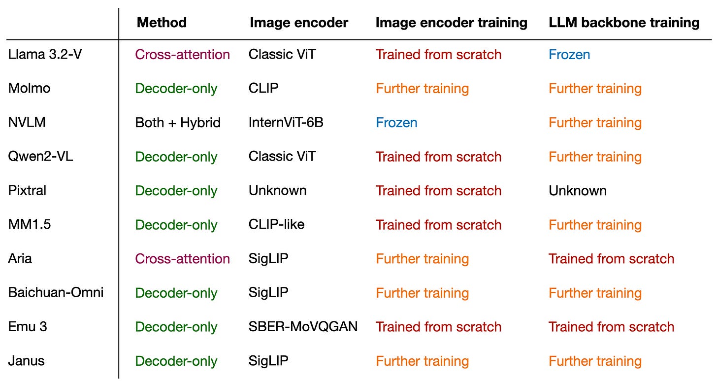
In any case, the main takeaway from this article is that multimodal LLMs can be built successfully in many different ways. Below is a figure that summarizes the different components of the models covered in this article.
I hope you found reading this article educational and now have a better understanding of how multimodal LLMs work!
This magazine is a personal passion project. For those who wish to support me, please consider purchasing a copy of my Build a Large Language Model (From Scratch) book. (I am confident that you'll get lots out of this book as it explains how LLMs work in a level of detail that is not found anywhere else.)

If you read the book and have a few minutes to spare, I'd really appreciate a brief review. It helps us authors a lot!
Alternatively, I also recently enabled the paid subscription option on Substack to support this magazine directly.
Your support means a great deal! Thank you!


Thank you for sharing it!
However, in the last "overview" diagram, the "Method" of Molmo and NVLM seems to be filled in incorrectly. That is, "Both + Hybrid" should correspond to NVLM instead of Molmo.
An excellent article to help me gain a full picture of multi modality