Finetuning Large Language Models

An introduction to the core ideas and approaches

Note: Last week, I was experimenting with posting articles outside the monthly Ahead of AI series that discusses the latest research and trends. Your positive response was very flattering. The article "Understanding Large Language Models — A Cross-Section of the Most Relevant Literature to Get Up to Speed" article received approximately ten times more likes than previous ones. This is incredibly motivating, and I will do my best to post more frequently than once a month, as time allows!

---

In the rapidly evolving field of artificial intelligence, utilizing large language models (LLMs) efficiently and effectively has become increasingly important. But we can use large language models in many different ways, which can be overwhelming if you are starting out.

In essence, we can use pretrained large language models for new tasks in two main ways: in-context learning and finetuning.

In this article, we will briefly go over what in-context learning means, and then we will go over the various ways we can finetune LLMs.

In-Context Learning and Indexing

Since GPT-2 (Radford et al.) and GPT-3 (Brown et al.), we have seen that generative large language models (LLMs) pretrained on a general text corpus are capable of in-context learning, which doesn’t require us to further train or finetune pretrained LLMs if we want to perform specific or new tasks that the LLM wasn’t explicitly trained on. Instead, we can directly provide a few examples of a target task via the input prompt, as illustrated in the example below.

An example of in-context learning.

In-context learning is very useful if we don’t have direct access to the model, for instance, if we are using the model through an API.

Related to in-context learning is the concept of hard prompt tuning where we modify the inputs in hope to improve the outputs as illustrated below.

An illustration of (hard) prompt tuning

By the way, we call it hard prompt tuning because we are modifying the input words or tokens directly. Later on, we will discuss a differentiable version referred to as soft prompt tuning (or often just called prompt tuning).

The prompt tuning approach mentioned above offers a more resource-efficient alternative to parameter finetuning. However, its performance typically falls short of finetuning, as it doesn't update the model's parameters for a specific task, which may limit its adaptability to task-specific nuances. Moreover, prompt tuning can be labor-intensive, as it often demands human involvement in comparing the quality of different prompts.

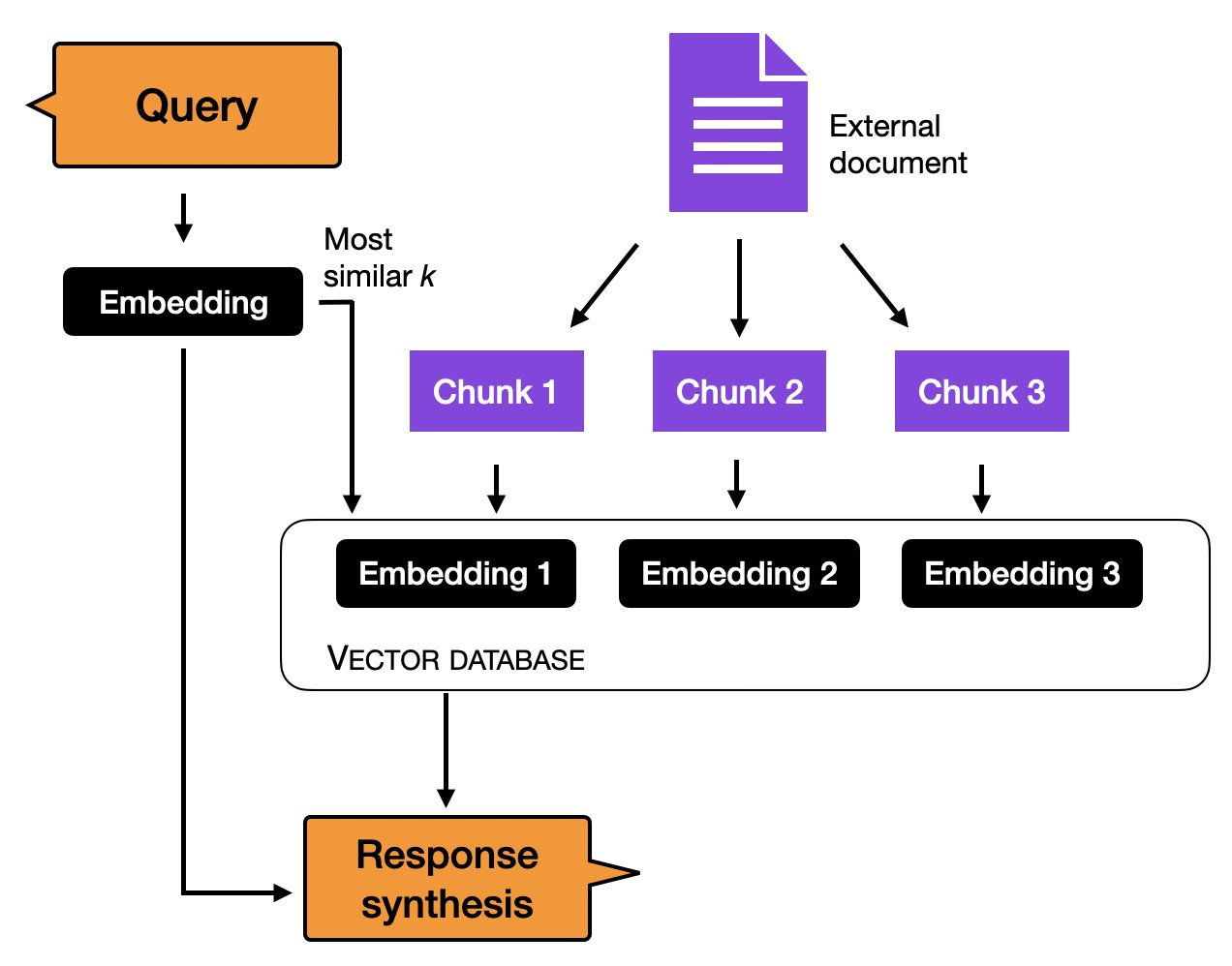
Before we discuss finetuning in more detail, another method to utilize a purely in-context learning-based approach is indexing. Within the realm of LLMs, indexing can be seen as an in-context learning workaround that enables the conversion of LLMs into information retrieval systems for extracting data from external resources and websites. In this process, an indexing module breaks down a document or website into smaller segments, converting them into vectors that can be stored in a vector database. Then, when a user submits a query, the indexing module calculates the vector similarity between the embedded query and each vector in the database. Ultimately, the indexing module fetches the top k most similar embeddings to generate the response.

An illustration of indexing.

The 3 Conventional Feature-Based and Finetuning Approaches

In-context learning is a valuable and user-friendly method for situations where direct access to the large language model (LLM) is limited, such as when interacting with the LLM through an API or user interface.

However, if we have access to the LLM, adapting and finetuning it on a target task using data from a target domain usually leads to superior results. So, how can we adapt a model to a target task? There are three conventional approaches outlined in the figure below.

The 3 conventional feature-based and finetuning approaches.

To provide some practical context for the discussions below, we are finetuning an encoder-style LLM such as BERT (Devlin et al. 2018) for a classification task. (To keep things simple, this classification task predicts whether a movie review has a positive or negative sentiment.) Note that instead of finetuning an encoder-style LLM, the same approach would work for GPT-like decoder-style LLMs, and I will provide an example of this in a future article. Furthermore, we can also finetuning decoder-style LLMs to generate multiple-sentence answers to specific instructions instead of just classifying texts. Also, for this, I will provide hands-on examples in future articles.

1) Feature-Based Approach

In the feature-based approach, we load a pretrained LLM and apply it to our target dataset. Here, we are particularly interested in generating the output embeddings for the training set, which we can use as input features to train a classification model. While this approach is particularly common for embedding-focused like BERT, we can also extract embeddings from generative GPT-style model.

The classification model can then be a logistic regression model, a random forest, or XGBoost – whatever our hearts desire. (However, based on my experience, linear classifiers like logistic regression perform best here.)

Conceptually, we can illustrate the feature-based approach with the following code:

model = AutoModel.from_pretrained("distilbert-base-uncased")

# ...
# tokenize dataset
# ...

# generate embeddings
@torch.inference_mode()
def get_output_embeddings(batch): 
    output = model(
        batch["input_ids"],
        attention_mask=batch["attention_mask"]
    ).last_hidden_state[:, 0]
return {"features": output}
  
dataset_features = dataset_tokenized.map(
  get_output_embeddings, batched=True, batch_size=10)

X_train = np.array(imdb_features["train"]["features"])
y_train = np.array(imdb_features["train"]["label"])

X_val = np.array(imdb_features["validation"]["features"])
y_val = np.array(imdb_features["validation"]["label"])

X_test = np.array(imdb_features["test"]["features"])
y_test = np.array(imdb_features["test"]["label"])

# train classifier
from sklearn.linear_model import LogisticRegression

clf = LogisticRegression()
clf.fit(X_train, y_train)

print("Training accuracy", clf.score(X_train, y_train))
print("Validation accuracy", clf.score(X_val, y_val))
print("test accuracy", clf.score(X_test, y_test))

(Interested readers can find the full code example here.)

2) Finetuning I – Updating The Output Layers

A popular approach related to the feature-based approach described above is finetuning the output layers (we will refer to this approach as finetuning I). Similar to the feature-based approach, we keep the parameters of the pretrained LLM frozen. We only train the newly added output layers, analogous to training a logistic regression classifier or small multilayer perceptron on the embedded features.

In code, this would look as follows:

model = AutoModelForSequenceClassification.from_pretrained(
    "distilbert-base-uncased",
     num_labels=2
) 

# freeze all layers
for param in model.parameters():
    param.requires_grad = False
    
# then unfreeze the two last layers (output layers)
for param in model.pre_classifier.parameters():
    param.requires_grad = True

for param in model.classifier.parameters():
    param.requires_grad = True
    
# finetune model
lightning_model = CustomLightningModule(model)

trainer = L.Trainer(
    max_epochs=3,
    ...
)

trainer.fit(
  model=lightning_model,
  train_dataloaders=train_loader,
  val_dataloaders=val_loader)

# evaluate model
trainer.test(lightning_model, dataloaders=test_loader)

(Interested readers can find the complete code example here.)

In theory, this approach should perform similarly well, in terms of modeling performance and speed, as the feature-based approach since we use the same frozen backbone model. However, since the feature-based approach makes it slightly easier to pre-compute and store the embedded features for the training dataset, the feature-based approach may be more convenient for specific practical scenarios.

3) Finetuning II – Updating All Layers

While the original BERT paper (Devlin et al.) reported that finetuning only the output layer can result in modeling performance comparable to finetuning all layers, which is substantially more expensive since more parameters are involved. For instance, a BERT base model has approximately 110 million parameters. However, the final layer of a BERT base model for binary classification consists of merely 1,500 parameters. Furthermore, the last two layers of a BERT base model account for 60,000 parameters – that’s only around 0.6% of the total model size.

Our mileage will vary based on how similar our target task and target domain is to the dataset the model was pretrained on. But in practice, finetuning all layers almost always results in superior modeling performance.

So, when optimizing the modeling performance, the gold standard for using pretrained LLMs is to update all layers (here referred to as finetuning II). Conceptually finetuning II is very similar to finetuning I. The only difference is that we do not freeze the parameters of the pretrained LLM but finetune them as well:

model = AutoModelForSequenceClassification.from_pretrained(
    "distilbert-base-uncased",
     num_labels=2
) 

# freeze layers (which we don't do here)
# for param in model.parameters():
#    param.requires_grad = False
    

# finetune model
lightning_model = LightningModel(model)

trainer = L.Trainer(
    max_epochs=3,
    ...
)

trainer.fit(
  model=lightning_model,
  train_dataloaders=train_loader,
  val_dataloaders=val_loader)

# evaluate model
trainer.test(lightning_model, dataloaders=test_loader)

(Interested readers can find the complete code example here.)

If you are curious about some real-world results, the code snippets above were used to train a movie review classifier using a pretrained DistilBERT base model (you can access the code notebooks here):

• 1) Feature-based approach with logistic regression: 83% test accuracy

• 2) Finetuning I, updating the last 2 layers: 87% accuracy

• 3) Finetuning II, updating all layers: 92% accuracy.

These results are consistent with the general rule of thumb that finetuning more layers often results in better performance, but it comes with increased cost.

Rule-of-thumb computational and modeling performance trade-offs for various approaches.

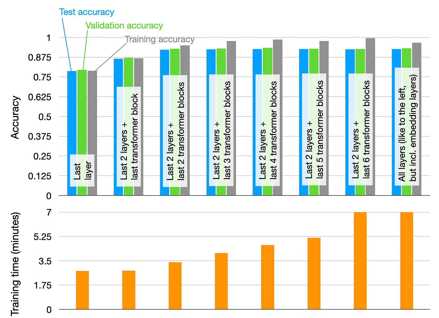
The scenarios above highlighted the three most distinct or extreme cases of finetuning: training only the last layer(s) versus training all layers. Of course, our mileage may vary based on the model and dataset, but exploring the various options in between may also be worthwhile. For instance, we can sometimes get the same modeling performance by training only half of the model (but more on parameter-efficient finetuning in the next section). For those who are curious, the figure below shows the predictive performances and training times for a DistilBERT model finetuned on the 20k training examples from the IMDB movie review dataset.

Performance of pretrained DistilBERT models finetuned on the IMDB Movie review dataset. The code can be found here on GitHub.

As we can see, training the last layer is the fastest but also results in the poorest modeling performance. As expected, training more layers improves the modeling performance but it also increases the computational cost. Most interestingly, we can see the predictive performance saturate when training the two fully connected output layers and the last two transformer blocks (the third block from the left). So, in this particular case (that is, for this particular model and dataset combination), it seems computationally wasteful to train more than these layers.

Parameter-Efficient Finetuning

Parameter-efficient finetuning allows us to reuse pretrained models while minimizing the computational and resource footprints. In sum, parameter-efficient finetuning is useful for at least 5 reasons:

1. Reduced computational costs (requires fewer GPUs and GPU time);

2. Faster training times (finishes training faster);

3. Lower hardware requirements (works with smaller GPUs & less smemory);

4. Better modeling performance (reduces overfitting);

5. Less storage (majority of weights can be shared across different tasks).

In the previous sections, we learned that finetuning more layers usually leads to better results. Now, the experiments above are based on a DistilBERT model, which is relatively small. What if we want to finetune larger models that only barely fit into GPU memory, for example, the latest generative LLMs? We can use the feature-based or finetuning I approach above, of course. But suppose we want to get a similar modeling quality as finetuning II?

Over the years, researchers developed several techniques (Lialin et al.) to finetune LLM with high modeling performance while only requiring the training of only a small number of parameters. These methods are usually referred to as parameter-efficient finetuning techniques (PEFT).

Some of the most widely used PEFT techniques are summarized in the figure below.

A selection of the most popular parameter-efficient finetuning techniques.

So, how do these techniques work? In a nutshell, they all involve introducing a small number of additional parameters that we finetuned (as opposed to finetuning all layers as we did in the Finetuning II approach above). In a sense, Finetuning I (only finetuning the last layer) could also be considered a parameter-efficient finetuning technique. However, techniques such as prefix tuning, adapters, and low-rank adaptation, all of which “modify” multiple layers, achieve much better predictive performance (at a low cost).

Since this is already a very long article, and since these are super interesting techniques, I will cover these techniques separately in the future.

Reinforcement Learning with Human Feedback

In Reinforcement Learning with Human Feedback (RLHF), a pretrained model is finetuned using a combination of supervised learning and reinforcement learning -- the approach was popularized by the original ChatGPT model, which was in turn based on InstructGPT (Ouyang et al.).

In RLHF, human feedback is collected by having humans rank or rate different model outputs, providing a reward signal. The collected reward labels can then be used to train a reward model that is then in turn used to guide the LLMs adaptation to human preferences.

The reward model itself is learned via supervised learning (typically using a pretrained LLM as base model). Next, the reward model is used to update the pretrained LLM that is to be adapted to human preferences -- the training uses a flavor of reinforcement learning called proximal policy optimization (Schulman et al.).

Screenshot from the InstructGPT paper outlining the RLHF process.

Why use a reward model instead of training the pretained model on the human feedback directly? That's because involving humans in the learning process would create a bottleneck since we cannot obtain feedback in real-time.

As mentioned above, the article is already very long, so I am deferring a more detailed explanation to a future article.

Conclusion

Fine-tuning all layers of a pretrained LLM remains the gold standard for adapting to new target tasks, but there are several efficient alternatives for using pretrained transformers. Methods such as feature-based approaches, in-context learning, and parameter-efficient finetuning techniques enable effective application of LLMs to new tasks while minimizing computational costs and resources.

Moreover, reinforcement learning with human feedback (RLHF) serves as an alternative to supervised finetuning, potentially enhancing model performance.

---

This magazine is a personal passion project that does not offer direct compensation. However, for those who wish to support me, please consider purchasing a copy of one of my books. If you find them insightful and beneficial, please feel free to recommend them to your friends and colleagues.

Machine Learning with PyTorch and Scikit-Learn, Machine Learning Q and AI, and Build a Large Language Model (from Scratch)

Your support means a great deal! Thank you!